Data fusion - GeoFIS

1. Basic concepts

Information fusion is done with a specific goal: for instance parameter estimation according to various sensors or risk level evaluation according to different sources of information. The objective is to compare different alternatives, locations, sites or zones, in the case of spatial data, according to the whole information.

Only values in the same scale and with the same meaning can be aggregated. The most popular aggregation operator is the weighted mean. When the data are of same kind, like in sensor fusion, there is no problem. This is not true in the general case.

Main steps:

criterion: attribute with a preference relation
from raw data to satisfaction degrees
aggregation of satisfaction degrees: score
comparison: $\mathbf{a \succ b \iff \psi(a) > \psi(b)}$

$\mathbf{(a_1, \ldots, a_n)}$ $\mathbf{, (b_1, \ldots, b_n)}$	$\mathbf{\overset{A}{\longrightarrow}}$	$\mathbf{\psi (a)}$ $\mathbf{, \psi (b)}$
$\uparrow$		$\mathbf{\scshape{c} \downarrow}$
$\mathbf{(x_1, \ldots, x_n)}$ $\mathbf{, (y_1, \ldots, y_n)}$		$\mathbf{\underset{\sim}{\prec} (a,b)}$

1.1 From raw data to satisfaction degrees

This step is mandatory to aggregate information sources in different scales and different units.

Criterion: if one wants to purchase a car, one of the attributes can be the time to reach a given speed, e. g. $100 km/h$ , from scratch. If the user prefers a fast car, then this time should be minimized. The acceleration time is an attribute of a car, the criterion of a fast car is better satisfied when this time is low.
Satisfaction degrees: the transformation of raw data into satisfaction degrees is done using a function. Figure 1 shows an example for the acceleration time.

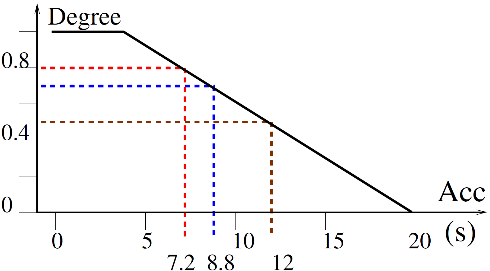
Figure 1

To each of the possible values for the attribute corresponds a degree in a commensurable scale, meaning that all the degrees, for all the attributes, are in the same range, e. g. the unit interval $[0,1]$ , and have the same meaning, $0$ when the criterion is not at all satisfied, for all $t>20s$ in this example, $1$ when it is fully satisfied, $t<4s$ in the example.

1.2 Aggregation of the degrees in the same scale and with the same meaning

Once the values from the $n$ information sources are converted into $n$ satisfaction degrees for each alternative, a car in our example, the next step is to summarize the $n$ values into a single one to ease the comparison between alternatives.

1.2.1 Numerical operators

Among the suitable properties for the aggregation operators are the idempotence, monotony and compromise: $\underset{i}{min} \ a_i \le \psi(a_1, \ldots, a_n) \le \underset{i}{max} \ a_i$

Two families of such operators are available in GeoFIS:

Weighted Arithmetic Mean (WAM)
$\psi(a_1, \ldots, a_n)= \sum_{i=1}^n w_ia_i, \quad w_i \in [0,1], \sum_{i=1}^n w_i=1$
Ordered Weighted Average (OWA)
$\psi(a_1, \ldots, a_n)= \sum_{i=1}^n w_ia_{(i)}, \quad w_i \in [0,1], \sum_{i=1}^n w_i=1$

$(.)$ : permutation such as $a_{(1)}\le \cdots \le a_{(n)}$

With the WAM, the weights are assigned to the information sources. This is not the case for the OWA: as the degrees are ordered the weights are assigned to the locations in the distribution, from the minimum to the maximum, whatever the information sources.

1.2.2 Aggregation using linguistic rules

Linguistic rules are used within fuzzy inference systems for approximate reasoning. The reader may refer to the Elementary fuzzy logic glossary for the basics of fuzzy logic and fuzzy inference systems and to the FisPro open source software for a user friendly interface for fuzzy inference system design and optimization.

As an example, consider the aggregation of three information sources to define the potential to increase production (yield):

Inputs			Outputs
CropLoad [3]	Eca [2]	Prun Wt [2]	Short term	Long term [3]
Average	Low	High	0.6	Low

There are three input variables, CropLoad, Eca and Pruning Weight, and two output ones, short and long term. The short term output uses a numerical values while the long term ones uses linguistic labels.

The numbers in brackets in the first row give the number of linguistic terms used for a given input or output variable: 3 for CropLoad and 2 for Eca, for instance. This number defines the granularity of the partition of the considered variable. The proposed labels are: Low, Average and High when 3 terms are used, Low and High when only 2 are needed.

The maximum number of rules is given by the product of the input granularities. In this example: $3 \times 2 \times 2 = 12$ .

The second row shows a rule that can also be expressed in natural language:

IF Cropload is Average and soil electrical conductivity is Low and Pruning Weight is High THEN Short term potential is 0.6 and Long term potential is Low

The final result is the given by the aggregation of all the rules for each of the output variables.

The third row shows the function used to turn raw data into satisfaction degrees. To a low CropLoad value corresponds a high degree for potential to increase production.

2. GeoFIS implementation

In the current version all the attributes must belong to the same layer. To be used in the fusion module an attribute must be selected as an input and a function to turn raw data to satisfaction degree has to be defined.
Four types of membership functions (Mf) are proposed:

Semi trapezoidal inf: low values are preferred
Semi trapezoidal sup: high values are preferred
Trapezoidal: around an interval
Triangular: about a value

The aggregation is available as a new variable, which can also be used as an input for another aggregation step, yielding a hierarchical structure.

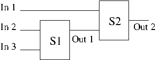
An aggregation operator is defined for each aggregated variable. Three are currently available:

WAM: the weights are assigned to the information sources
OWA: the weights are given to the position in the distribution
FIS: a fuzzy inference system (FIS) including linguistic rules

To define the rule base the granularity can be edited and then the corresponding labels are proposed for rule definition. All the possible rules can also be generated, the user has to set the corresponding conclusion, either numerical of fuzzy.

Finally, the FIS is automatically generated from the rule base and stored in a file (.fis) to be load as a parameter. It can also be edited using FisPro.

Weigth learning (WAM or OWA)

To learn the weigths, the target (learning variable) must range in the unit interval.
A min-max standardization is applied: $\displaystyle x \rightarrow \frac{x-min}{max-min}$

The proposed values depend on the target range:

min=0 and max=1 if the range is included in the unit interval
the min and max of the target otherwise

Only values that include the target range are valid.

References

S. Guillaume, T. Bates, J. Lablée, T. Betts, and J. Taylor, “Combining spatial data layers using fuzzy inference systems: application to an agronomic case study,” in Proceedings of the 6th international conference on geographical information systems theory, applications and management (gistam 2020), Prague, Czech Republic, 2020, pp. 62-71.
[Bibtex]

@Inproceedings{gistam20,
author = {Serge Guillaume and Terry Bates and Jean-Luc Labl\'ee and Thom Betts and James Taylor},
title = {Combining Spatial Data Layers Using Fuzzy Inference Systems: Application to an Agronomic Case Study},
year = {2020},
month = {May},
booktitle = {Proceedings of the 6th International Conference on Geographical Information Systems Theory, Applications and Management (GISTAM 2020)},
pages = {62-71},
publisher = {SCITEPRESS},
address = {Prague, Czech Republic},
isbn = {978-989-758-425-1},
doi = {10.5220/0009356000620071},
}

D. Y. Mora-Herrera, S. Guillaume, D. Snoeck, and O. Zúñiga Escobar, “A fuzzy logic based soil chemical quality index for cacao,” Computers and electronics in agriculture, vol. 177, p. 105624, 2020.
[Bibtex]

@article{denys20,
author = {Denys Yohana Mora-Herrera and Serge Guillaume and Didier Snoeck and Orlando {Z\'u{\~n}iga Escobar}},
title = {A fuzzy logic based soil chemical quality index for cacao},
journal = {Computers and Electronics in Agriculture},
volume = {177},
year = {2020},
pages = {105624},
doi = {10.1016/j.compag.2020.105624},
}